Stock Return Example

Introduction and import data

In finance, the return of a stock (or index) is the following: if the value today was 11 and the value yesterday was 10, the return is 11/10 = 1.10, or 10% growth. The logarithmic return is then log(11/10)=0.0953. Since log(1)=0, a positive log returns indicate growth, and negative log returns indicate loss. In this study, let's focus on first percentile of the stock return distribution, Q(0.01)Q(0.01). The returns will be larger than this 99% of the time, so Q(0.01)Q(0.01) gives an idea of how bad the bad performance will be, which is useful for planning.

Let's first import the data file, take the last column (containing the daily closing price), and calculate the logarithmic returns based only on the closing price. Note that the file is in reverse chronological order (newest first).

tmp1 <- read.csv("SPdata.csv",header=T)
tmp2 <- log(rev(tmp1[,7]))
lgrn <- diff(tmp2) #log-return
par(mar=c(5,5,4,1),cex.main=1.5,cex.axis=1.3,cex.lab=1.4)
plot(lgrn,type="l")

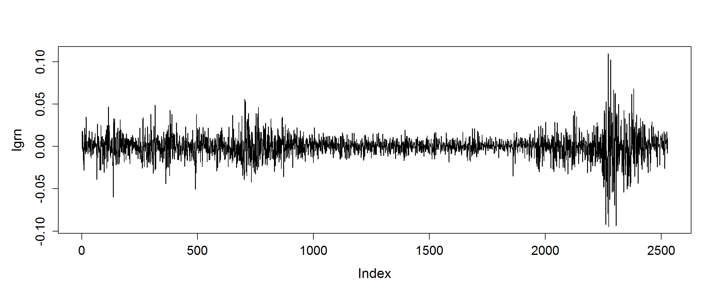
summary(lgrn)

##       Min.    1st Qu.     Median       Mean    3rd Qu.       Max. 
## -9.470e-02 -6.441e-03  4.668e-04 -6.404e-05  6.309e-03  1.096e-01

Gaussian Model

In many applications in finance, it is common to model daily returns as independent Gaussian variables. Let's first find the best-fitting Gaussian distribution, which has the same mean and standard deviation as the ones from the log-return data.

N <- length(lgrn)
mu.obs <- mean(lgrn)
sd.obs <- sqrt(var(lgrn)*(N-1)/N)
#Q.01: the first percentile from the best-fitting normal distribution
Q.01 <- qnorm(p = 0.01, mean = mu.obs, sd = sd.obs) 
mu.obs #mean of log-return

## [1] -6.404402e-05

sd.obs #standard deviation of log-return

## [1] 0.01399881

Q.01

## [1] -0.03263014

Now, let's generate simulated data from the Gaussian model and investigate the uncertainty for Q(0.01)Q(0.01). sim is a function which simulates a dataset from a normal distribution with specified mean and SD, and returns the sample mean and SD. q0.01 is a function to find the first percentile of a normal distribution with specified mean and SD.

sim <- function(m, s, n){
  tmp1 <- rnorm(n, mean=m, sd=s)
  tmp2 <- mean(tmp1)
  tmp3 <- sd(tmp1)
  out <- list(mean=tmp2, sd=tmp3)
  return(out)
}

q0.01 <- function(mean.sd.list){
  out <- qnorm(p=0.01, mean.sd.list$mean, mean.sd.list$sd)
  return(out)
}

Here is the game plan.

1. First, we randomly sample NN (sample size from original data) data points from the best-fitting normal distribution.
2. Then, we calculate the sample mean and SD from the simulated data.
3. Output the first percentile of the normal distribution with the mean and SD calculated in Step 2.
4. Repeat Step 1-3 5,000 times.
5. Calculate the 95% confidence interval from the output 5,000 first percentiles.

iter <- 5000
res <- rep(0,iter)
for (it in 1:iter){
  tmp1 <- sim(mu.obs,sd.obs,N)
  res[it] <- q0.01(tmp1)
}
quantile(res,prob=c(0.025,0.975))

##        2.5%       97.5% 
## -0.03366107 -0.03159475

Let's compare the computed CI with the Q(0.01)Q(0.01) from the original data.

quantile(lgrn,prob=0.01)

##          1% 
## -0.03923286

It is surprising to see that the first percentile from the original data is not even close to the computed confidence interval! Why? Let's check the distribution of the log-return data.

par(mar=c(5,5,4,1),cex.main=1.5,cex.axis=1.3,cex.lab=1.4)
plot(density(lgrn), lwd = 2,
  main = "Fitting a kernel density (black solid) and the best-fitting 
          normal pdf (red dashed) to log returns",
  xlab = "log returns", ylab = "density")
curve(dnorm(x,mean = mu.obs, sd = sd.obs),add=TRUE,col="red",lwd=2.4,lty=2)

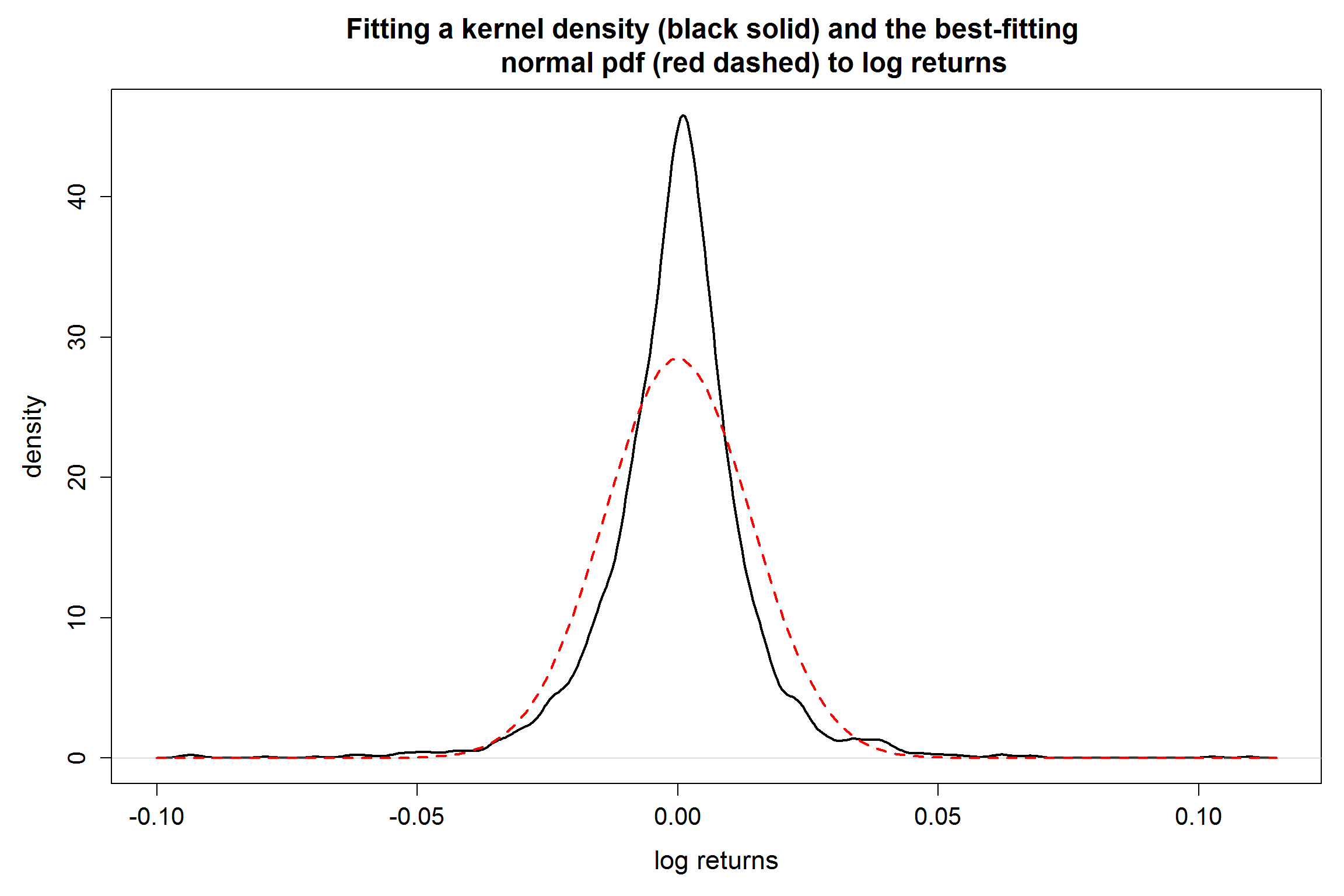
From the density plots, we see that the log-return does NOT follow a normal distribution.

Bootstrapping approach

Now let's use the bootstrapping to solve the problem.

1. First, we randomly sample N data points with replacement from the original data.
2. Then, we output the first percentile of the bootstrap sample.
3. Repeat Step 1-2 5,000 times.
4. Calculate the 95% confidence interval from the output 5,000 first percentiles.

iter <- 5000
res2 <- rep(0,iter)
for (it in 1:iter){
  set.seed(it)
  res2[it] <- quantile(lgrn[sample(1:N,size=N,replace=T)],prob=0.01)
}
quantile(res2,prob=c(0.025,0.975)) #95% bootstrap interval

##        2.5%       97.5% 
## -0.04774186 -0.03468522

quantile(lgrn,prob=0.01) #first percentile from original data

##          1% 
## -0.03923286

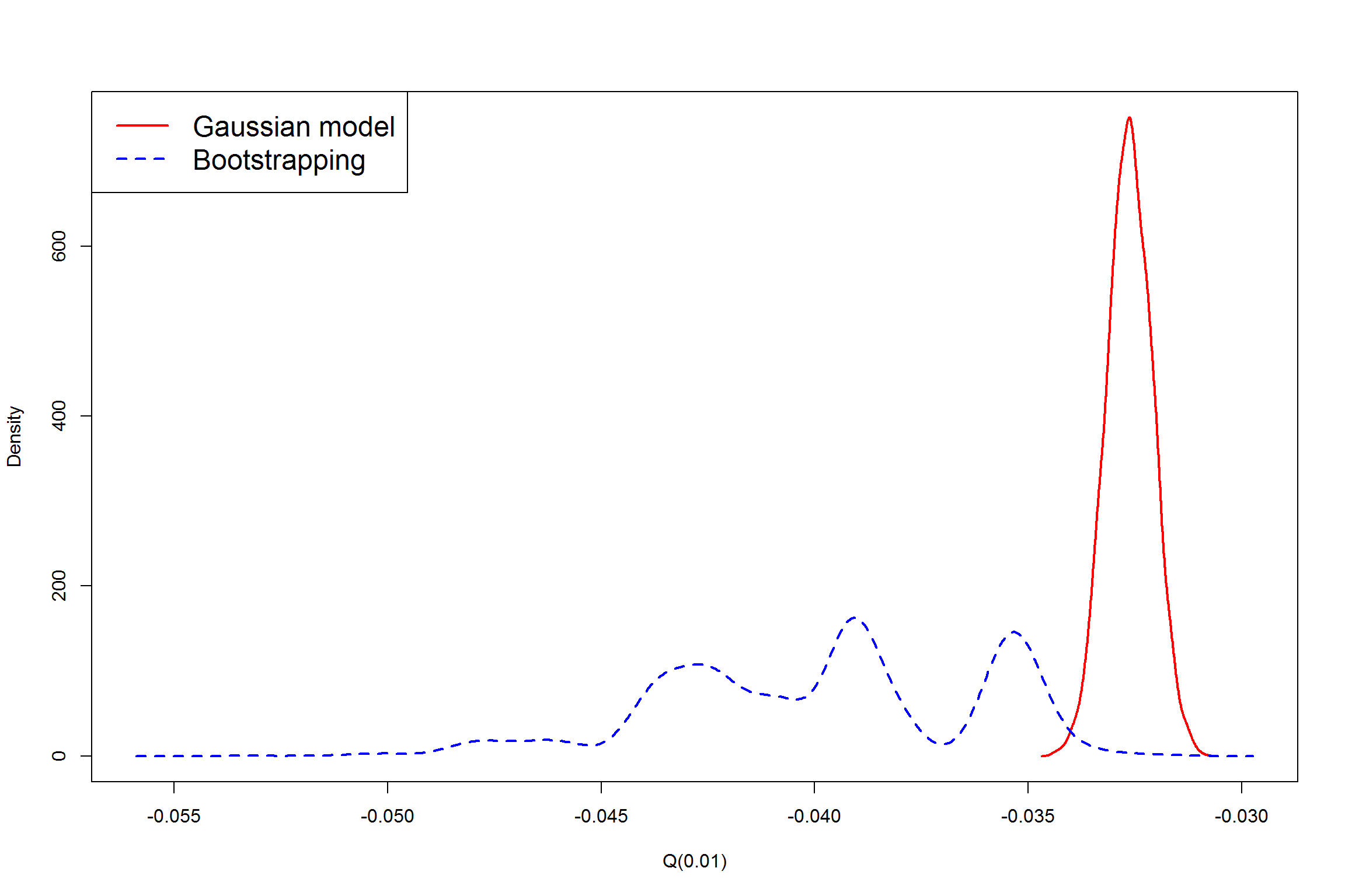
We see the 95% bootstrap interval holds the Q(0.01)Q(0.01) from the original data. Let's check one more thing: the sampling distribution of Q(0.01)Q(0.01) under Gaussian model and empirical distribution from bootstrapping.

a=density(res) #Density of Q(0.01) under normal assumption
b=density(res2)#Density of Q(0.01) from bootstrapping
plot(a$x,a$y,xlab="Q(0.01)",ylab="Density",main="",type="l",
     xlim=range(a$x,b$x),ylim=range(a$y,a$y),lwd=2,col="red")
lines(b$x,b$y,lwd=2,lty=2,col="blue")
legend("topleft",c("Gaussian model","Bootstrapping"),lty=c(1,2),lwd=2,col=c("red","blue"),cex=1.5)