Model Assessment

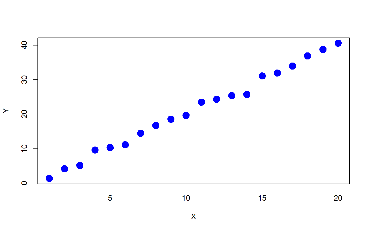
First, let’s generate a simple simulation example with \(x=1,2,\cdots,20\) and \(y\) is a linear function of \(x\) with some additive random noise:

\[ y_i=2x_i+\epsilon_i, \quad \epsilon \sim N(0,1). \]

n=20
x=1:n
set.seed(1)
e=rnorm(n,mean=0,sd=1)
y=x*2+e
plot(x,y,xlab="X",ylab="Y",pch=19,col="blue",cex=2)

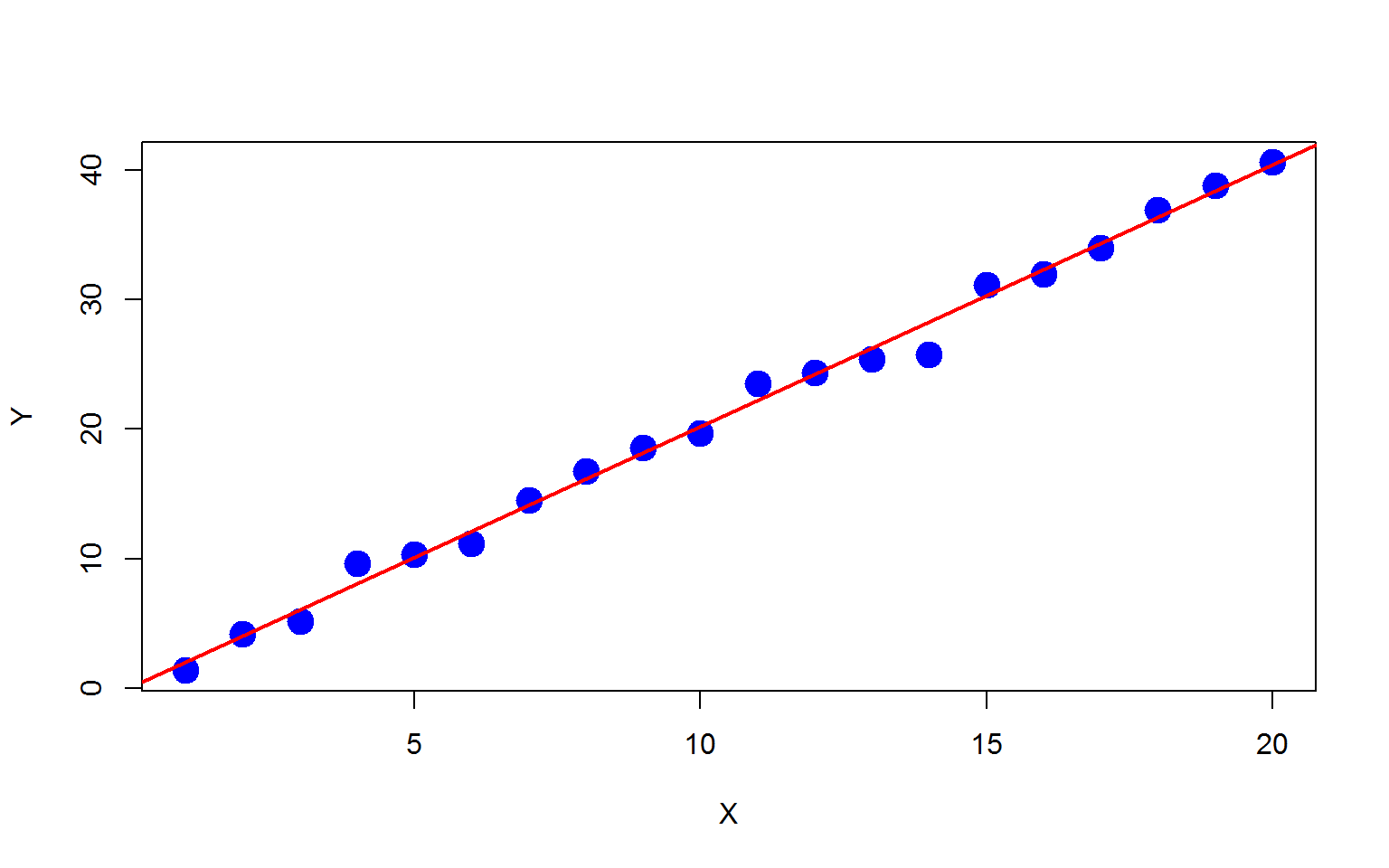
Then we fit a simple linear regression on the dataset.

f=lm(y~x)
plot(x,y,xlab="X",ylab="Y",pch=19,col="blue",cex=2)
abline(f,col="red",lwd=2)

f$fit

##         1         2         3         4         5         6         7 
##  1.985490  4.007072  6.028655  8.050237 10.071820 12.093402 14.114985 
##         8         9        10        11        12        13        14 
## 16.136568 18.158150 20.179733 22.201315 24.222898 26.244480 28.266063 
##        15        16        17        18        19        20 
## 30.287645 32.309228 34.330810 36.352393 38.373976 40.395558

f$residual

##          1          2          3          4          5          6 
## -0.6119435  0.1765711 -0.8642834  1.5450435  0.2576879 -0.9138708 
##          7          8          9         10         11         12 
##  0.3724441  0.6017572  0.4176313 -0.4851210  1.3104660  0.1669455 
##         13         14         15         16         17         18 
## -0.8657208 -2.4807627  0.8372856 -0.3541615 -0.3470007  0.5914432 
##         19         20 
##  0.4472457  0.1983433

mean(f$residual^2) #MSE on training set

## [1] 0.7768427

In-sample Optimism

The MSE on the training set is obviously smaller than the true value (since this is a simulation example, we do know the MSE.

set.seed(2)
e2=rnorm(n,mean=0,sd=1)
y2=x*2+e2
mean((y2-f$fit)^2) #MSE on new responses

## [1] 1.061651

You can see that the MSE on the training set is too optimistic. Now let’s find out the expected loss on the training samples for new response values \[ \frac{1}{n}\sum_{i=1}^n E_{Y^0}\left [ L(Y_i^0, \hat{f}(x_i))|\mathcal{T}\right ]. \]

 

iter=1000
mse=rep(0,iter)
for (i in 1:iter){
  set.seed(i+1)
  e3=rnorm(n,mean=0,sd=1)
  y3=x*2+e3
  mse[i]=mean((y3-f$fit)^2)
}
mean(mse) #Estimate of the expected loss on training set with new Ys

## [1] 1.043732

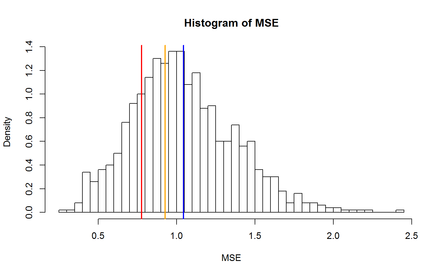
hist(mse,nclass=50,xlab="MSE",ylab="Density",freq=F,main="Histogram of MSE")
abline(v=mean(f$residual^2),col="red",lwd=2)
abline(v=mean(mse),col="blue",lwd=2)

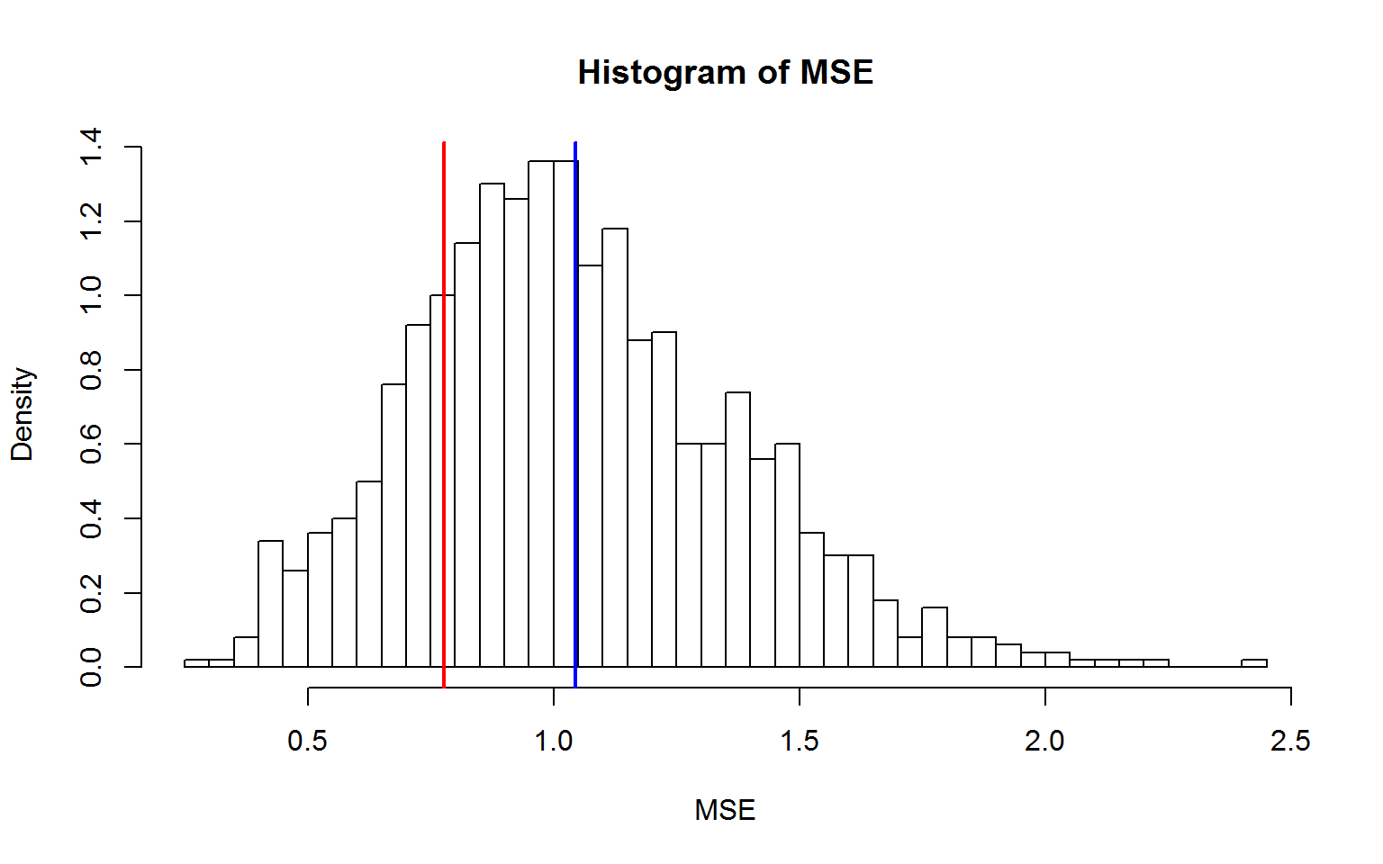In-sample optimism is defined as the difference between the expected loss on the training samples for new response values and the training error

\[
 
op=\frac{1}{n}\sum_{i=1}^n E_{Y^0}\left [ L(Y_i^0, \hat{f}(x_i))|\mathcal{T}\right ] - \overline{err}.
 
\]

If we can find out the in-sample optimism, we can have a better estimate of the expected loss on the training samples for new response values.

\[
 
\frac{1}{n}\sum_{i=1}^n E_{Y^0}\left [ L(Y_i^0, \hat{f}(x_i))|\mathcal{T}\right ]=op+\overline{err}.
 
\]

#In-sample optimism
op=mean(mse)-mean(f$residual^2)
op

## [1] 0.2668894'

#A better estimate of performance on test x values
op+mean(f$residual^2)

## [1] 1.043732

Mallow Cp and AIC are developed based on the above idea with the fact that

\[
 
E_y(op)=\frac{2}{n} \sum_{i=1}^n Cov(\hat{y},y_i).
 
\]

K-fold Cross-validation

We can estimate the generalization performance through cross-validation. For linear models, we can easily calculate the leave-one-out CV without fitting models n times.

\[
 
\frac{1}{n}\sum_{i=1}^n [y_i-\hat{f}^{-i}(x_i)]^2 = \frac{1}{n}\sum_{i=1}^n \left[ \frac{y_i-\hat{f}(x_i)}{1-H_{ii}}\right ]^2, \quad where \quad \hat{f}=Hy.
 
\]

#Hat-diagonal values (leverage)
hat.diag=influence(f)$hat
#LOOCV: PRESS (predicted residual error sum of squares)
press=mean(((y-f$fit)/(1-hat.diag))^2)
press

## [1] 0.927807

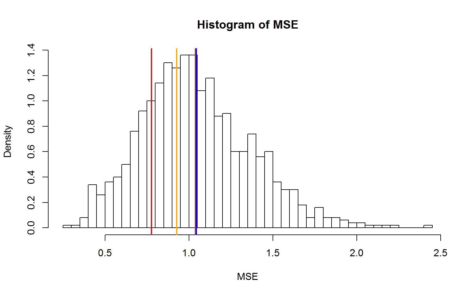
hist(mse,nclass=50,xlab="MSE",ylab="Density",freq=F,main="Histogram of MSE")
abline(v=mean(f$residual^2),col="red",lwd=2)
abline(v=mean(mse),col="blue",lwd=2)
abline(v=press,col="orange",lwd=2)

Out-of-bag (OOB) Samples in Bootstrapping

we can also use out-of-bag (OOB) samples in bootstrapping to estimate the generalization performance of a model. Let’s first see what the OOB samples are.

#Use Out-of-bag (OOB) estimate to evaluate performance
set.seed(1)
boot.id=sample(1:20,size=20,replace=T)
boot.id

##  [1]  6  8 12 19  5 18 19 14 13  2  5  4 14  8 16 10 15 20  8 16

setdiff(1:20,boot.id) #out-of-bag samples

## [1]  1  3  7  9 11 17

Let’s estimate the genalization performance of a model using OOB samples.

iter=1000
mse.boot=rep(0,iter)
for (i in 1:iter){
  set.seed(i+1)
  boot.id=sample(1:20,size=20,replace=T)
  f2=lm(y[boot.id]~x[boot.id])
  oob.id=setdiff(1:20,boot.id)
  y.hat=x[oob.id]*f2$coef[2]+f2$coef[1]
  mse.boot[i]=mean((y[oob.id]-y.hat)^2)
}
mean(mse.boot)

## [1] 1.039492

hist(mse,nclass=50,xlab="MSE",ylab="Density",freq=F,main="Histogram of MSE")
abline(v=mean(f$residual^2),col="red",lwd=2)
abline(v=mean(mse),col="blue",lwd=2)
abline(v=press,col="orange",lwd=2)
abline(v=mean(mse.boot),col="brown",lwd=2)